Понимание компромисса смещения
Дата публикации May 21, 2018
Всякий раз, когда мы обсуждаем прогнозирование модели, важно понимать ошибки прогнозирования (смещение и дисперсия). Существует компромисс между способностью модели минимизировать смещение и дисперсию. Получение правильного понимания этих ошибок поможет нам не только построить точные модели, но и избежать ошибки переоснащения и недостаточной подгонки.
Итак, давайте начнем с основ и посмотрим, как они влияют на наши модели машинного обучения.
Что такое уклон?
Что такое дисперсия?
Математически
Пусть переменная, которую мы пытаемся предсказать как Y, а другие ковариаты как X. Мы предполагаем, что между ними существует такая связь, что
Мы сделаем модель f ^ (X) для f (X), используя линейную регрессию или любую другую технику моделирования.
Таким образом, ожидаемая квадратная ошибка в точке х

Err (x) может быть далее разложен как

Смещение и дисперсия, используя диаграмму «бычий глаз»

В контролируемом обучении,underfittingпроисходит, когда модель не может захватить базовый шаблон данных. Эти модели обычно имеют высокий уклон и низкую дисперсию. Это происходит, когда у нас очень мало данных для построения точной модели или когда мы пытаемся построить линейную модель с нелинейными данными. Кроме того, такого рода модели очень просты для захвата сложных моделей в данных, таких как линейная и логистическая регрессия.
В контролируемом обучении,переобученияпроисходит, когда наша модель фиксирует шум вместе с базовым шаблоном в данных. Это происходит, когда мы много тренируемся в нашей модели из-за шумного набора данных. Эти модели имеют низкий уклон и высокую дисперсию. Эти модели очень сложны, как деревья решений, которые склонны к переоснащению.

Почему Bias Variance Tradeoff?
Если наша модель слишком проста и имеет очень мало параметров, то она может иметь высокое смещение и низкую дисперсию. С другой стороны, если наша модель имеет большое количество параметров, она будет иметь высокую дисперсию и низкое смещение. Таким образом, мы должны найти правильный / хороший баланс, не перегружая и не подбирая данные.
Этот компромисс между сложностью и является причиной компромисса между смещением и дисперсией. Алгоритм не может быть более сложным и менее сложным одновременно.
Общая ошибка
Чтобы построить хорошую модель, нам нужно найти хороший баланс между смещением и дисперсией, чтобы минимизировать общую ошибку.


Оптимальный баланс смещения и дисперсии никогда не будет соответствовать или не соответствовать модели.
Поэтому понимание предвзятости и дисперсии имеет решающее значение для понимания поведения моделей прогнозирования.
Анализ малых данных
КвазиНаучный блог Александра Дьяконова
Смещение (bias) и разброс (variance)
Сегодня дадим немного объяснений стандартных для машинного обучения понятий: смещение, разброс, переобучение и недообучение. Как всегда, всё объясним просто (но нужна будет математическая подготовка), на картинках, с примерами (в данном случае на модельных задачах). Все рисунки и эксперименты авторские, в конце, по традиции, изюминка – в чём при объяснении этих понятий Вас обманывают на курсах по ML и в учебниках;)

Ниже обсудим несколько фундаментальных понятий машинного обучения. Первое – переобучение (overfitting) – явление, когда ошибка на тестовой выборке заметно больше ошибки на обучающей. Это главная проблема машинного обучения: если бы такого эффекта не было (ошибка на тесте примерно совпадала с ошибкой на обучении), то всё обучение сводилось бы к минимизации ошибки на тесте (т.н. эмпирическому риску).
Второе – недообучение (underfitting) – явление, когда ошибка на обучающей выборке достаточно большая, часто говорят «не удаётся настроиться на выборку». Такой странный термин объясняется тем, что недообучение при настройке алгоритмов итерационными методами (например, нейронных сетей методом обратного распространения) можно наблюдать, когда сделано слишком маленькое число итераций, т.е. «не успели обучиться».
Третье – сложность (complexity) модели алгоритмов (допускает множество формализаций) – оценивает, насколько разнообразно семейство алгоритмов в модели с точки зрения их функциональных свойств (например, способности настраиваться на выборки). Повышение сложности (т.е. использование более сложных моделей) решает проблему недообучения и вызывает переобучение.
Сначала опишем на примере, как проявляется проблема выбора сложности и почему возникает переобучение. Для начала рассмотрим задачу регрессии. Для простоты будем считать, что это регрессия от одного признака x. Целевая зависимость y(x) известна в конечном наборе точек. На рис. 1 показана выборка для зависимости вида y = sin(4x) + шум, на рис. 2 для зашумлённой пороговой зависимости.
 Рис. 1. Настройка полиномов различных степеней на обучающую выборку.
  Рис. 2. Настройка полиномов различных степеней на обучающую выборку.
На рисунках показаны также решения указанных задач полиномиальной регрессией с разными степенями полиномов. Видно, что в обеих задачах полином первой степени явно плохо подходит для описания целевой зависимости, второй – достаточно хорошо её описывает, хотя ошибки есть и на обучающей выборке, седьмой – идеально проходит через точки обучающей выборки, но совсем не похож на «естественную функцию» и существенно отклоняется от целевой зависимости в остальных точках.
Если попробовать решить задачу полиномами различной степени, то мы получим рис. 3 (он построен для первой задачи, но во второй картина аналогичная). Видно, что с увеличением степени ошибка на обучающей выборке падает, а на тестовой (мы взяли очень мелкую сетку отрезка [0, 1]) – сначала падает, потом возрастает.
 Рис. 3. Зависимость ошибки на обучении и тесте от степени полинома.
Попробуем разобраться, в чём дело с теоретической точки зрения (сейчас немного математики). Наша целевая зависимость имеет вид

Мы строим алгоритм (в нашем случае полином фиксированной степени) a=a(x), посмотрим чему равно математическое ожидание квадрата отклонения ответа алгоритма от истинного значения:

Здесь важно понимать, как берутся матожидания (т.е., по сути, интегрирования) в приведённых выше формулах. Мы считаем, что обучающая выборка выбирается случайно из некоторого распределения, настроенный алгоритм тоже случаен, поскольку зависит от выборки, настройка алгоритма также может быть стохастической. Таким образом, матожидание берётся по всем данным (обучающим выборкам) и настройкам алгоритма, а сами формулы записываются в конкретной точке x:

При желании, можно проинтегрировать полученные формулы и по всем объектам (точнее, по какому-то распределению всех объектов) и получить уже смещение и разброс модели алгоритмов как таковой.
Разбросом (variance) мы назвали дисперсию ответов алгоритмов Da, а смещением (bias) – матожидание разности между истинным ответом и выданным алгоритмом: E(f – a). Мы получили, что ошибка раскладывается на три составляющие. Первая связана с шумом в самих данных, а вот две остальные связаны с используемой моделью алгоритмов. Понятно, что разброс характеризует разнообразие алгоритмов (из-за случайности обучающей выборки, в том числе шума, и стохастической природы настройки), а смещение – способность модели алгоритмов настраиваться на целевую зависимость. Проиллюстрируем это. На рис. 4-5 – показаны различные полиномы первой степени, они настроены на разных обучающих выборках. В точке x=0.5 ответы алгоритмов являются случайными величинами, они немного «разбросаны» (есть variance), а также они сильно смещены (есть bias) относительно правильного ответа (который, кстати, даже если нам и известен, то с точностью до шума).
 Рис. 4. Полиномы 1й степени, настроенные на разных обучающих выборках.
  Рис. 5. Шум, разброс и смещение при настройках полиномов 1й степени.
На рис. 6-7 изображены уже полиномы второй степени (настроенные на тех же выборках). В точке x=0.5 у них сильно меньше смещение и чуть меньше разброс. Видно, что они совсем неплохо описывают целевую зависимость во всех точках.
 Рис. 6. Полиномы 2й степени, настроенные на разных обучающих выборках.
  Рис. 7. Шум, разброс и смещение при настройках полиномов 2й степени.
 Рис. 8. Объяснение разброса и смещения на примере игры в дартс.
Ещё важный момент: спортсмен может повысить точность целясь выше/ниже/правее/левее, а для алгоритма нет таких понятий. Напомним, что разброс и смещение мы вводили в конкретной точке. Если изменить смещение в этой точке, то модель будет по-новому вести себя и в остальных. Если же усреднить смещение, точнее его квадрат, по всем точкам, то мы получим просто число (оно не указывает, как менять модель, чтобы уменьшить ошибку).
Теперь рассмотрим самую частую иллюстрацию, которую приводят при объяснении разброса и смещения, см. рис. 9. Она полностью согласуется с рис. 3. При увеличении сложности модели (например, степени полинома) ошибка на независимом контроле сначала падает, потом начинает увеличиваться. Обычно это связывают с уменьшением смещения (в сложных моделях очень много алгоритмов, поэтому наверняка найдутся те, которые хорошо описывают целевую зависимость) и увеличением разброса (в сложных моделях больше алгоритмов, а следовательно, и больше разброс).
 Рис. 9. Классическая иллюстрация изменения разброса и смещения.
Для простых моделей характерно недообучение (они слишком простые, не могут описать целевую зависимость и имеют большое смещение), для сложных – переобучение (алгоритмов в модели слишком много, при настройке мы выбираем ту, которая хорошо описывает обучающую выборку, но из-за сильного разброса она может допускать большую ошибку на тесте).
Теперь рассмотрим задачу классификации. Отметим, что для неё тоже есть результат о разложении ошибки на шум, разброс и смещение. На рис. 10-12 показаны результаты экспериментов в задаче с двумя классами (стандартная задача «два полумесяца») и моделью k ближайших соседей (kNN) при разных k. Результат также согласуется с рис. 9, если учесть, что изображена точность, а не ошибка, и сложность алгоритма
1/k. Возникает вопрос, а почему так вводится сложность для kNN? Ведь при разных k эти алгоритмы
Всё очень просто: часто сложность как раз и логично формализовать как 1/variance. На рис. 11 показаны разделяющие поверхности метода 1NN для разных выборок, которые описывают одну и ту же целевую зависимость. Они очень сильно отличаются друг от друга. А разделяющие поверхности kNN при больших k, см. рис 12, различаются существенно меньше. И чем выше k, тем стабильней результат. В этом смысле это очень простые алгоритмы: то, как они разделяют классы, меньше зависит от исходных данных, т.е. по определению ответ алгоритма 9NN в каждой точке зависит от 9и ближайших соседей, а по факту он практически не меняется от выборки к выборке (при варьировании обучения).
 Рис. 10. Точность метода kNN при разных k на обучении и контроле.
  Рис. 11. Разделяющие поверхности 1NN для разных выборок (одинаково распределённых).
  Рис. 12. Разделяющие поверхности 9NN для тех же выборок.
Теперь покажем, в чём не правы стандартные учебники и учебные курсы по машинному обучению. Проведём эксперименты по оцениванию разброса и смещения в модельных задачах. На рис. 13-14 приведены результаты для задачи с целевой зависимостью «ступенька», а на рис. 15-16 для задачи с целевой зависимостью «sin(4x)».
 Рис. 13. «Средние» полиномы различных степеней в задаче «ступенька».
  Рис. 14. Ошибка при разных степенях полиномов в задаче «ступенька».
  Рис. 15. «Средние» полиномы различных степеней в задаче «синус».
  Рис. 16. Ошибка при разных степенях полиномов в задаче «синус».
Очевидно, что степень полинома – очень естественная мера сложности для полиномиальной регрессии. Но полученные рисунки немного отличаются от рис. 9:
Почему так происходит? Одна их причин в том, что «сложность модели», если мы хотим видеть красивые графики монотонных и унимодальных функций, правильнее определять для конкретных данных! Например, ступенчатая функция нечётная (с точностью до смещения) и для восстановления такой целевой зависимости лучше подходят полиномы с нечётной старшей степенью.
Кстати, если использовать полиномиальную регрессию с L2-регуляризацией, то на рис. 16 смещение начинает вести себя «по классике»: убывать при увеличении степени полинома.
П.С. Дальше возникают естественные вопросы: как найти оптимальную сложность модели, как решать задачу сложными моделями и не переобучаться (используют же нейросети). Но это тема для отдельного поста… Просьба к читателям – давать отклики в комментариях. Этот материал будет использован, в том числе, в рамках нового курса на ВМК МГУ, а также в книжке, которую автор уже и не надеется закончить… Поэтому любые замечания по формулировкам, корректности выводов и т.п. будут полезны. Удачи!
Bias-Variance Trade-off in DataScience and Calculating with Python

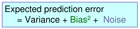
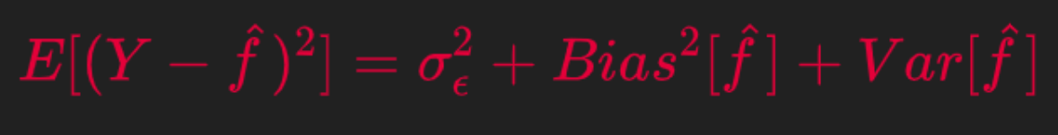
The target of this blog post is to discuss the concept around and the Mathematics behind the below formulation of Bias-Variance Tradeoff.
And in super simple term
Total Prediction Error = Bias + Variance
The goal of any supervised machine learning model is to best estimate the mapping function (f) for the output/dependent variable (Y) given the input/independent variable (X). The mapping function is often called the target function because it is the function that a given supervised machine learning algorithm aims to approximate.
The Expected Prediction Error for any machine learning algorithm can be broken down into three parts:
Bias Error
Variance Error
Irreducible Error
Why at all we need for MSE (Mean Squared Error) for training and testing datasets separately
Exploring these in detail is very important to understand the whole concepts around the Bias-Variance tradeoff.
Training and testing datasets have different purposes.
The training set trains the model how to predict the dependent variable values and we derive the Estimator equation from the training dataset. While, the testing datasets are there for testing the Estimator equation on how good an estimator they are really.
Now lets examine this in depth.
In the regression setting, the most commonly-used measure is the mean squared error (MSE), is given by
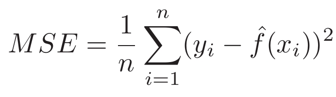
where f ˆ (x i) is the prediction that f ˆ gives for the i-th observation. The MSE
will be small if the predicted responses are very close to the true responses, and will be large if for some of the observations, the predicted and true responses differ substantially. The Test-MSE Equation is computed using the training data that was used to fit the model, and so should more accurately be referred to as the training MSE. But in general, we do not really care how well the method works training on the training data. Rather, we are interested in the accuracy of the predictions that we obtain when we apply our method to previously unseen test data.
Why is this what we care about? Suppose that we are interested test data in developing an algorithm to predict a stock’s price based on previous stock returns. We can train the method using stock returns from the past 6 months. But we don’t really care how well our method predicts last week’s stock price. We instead care about how well it will predict tomorrow’s price or next month’s price.


Instead, we want to know whether fˆ(x0 ) (i.e. the estimated target value based on a test-data input) is approximately equal to y0, where (x0, y0 ) is a previously unseen test observation not used to train the statistical learning method. We want to choose the method that gives the lowest test MSE, as opposed to the lowest training MSE. In other words, if we had a large number of test observations, we could compute

But what if no test observations are available? In that case, one might imagine simply selecting a statistical learning method that minimizes
the training MSE. Unfortunately, this strategy does not work. There is no guarantee that the method with the lowest training MSE will also have the lowest test MSE.
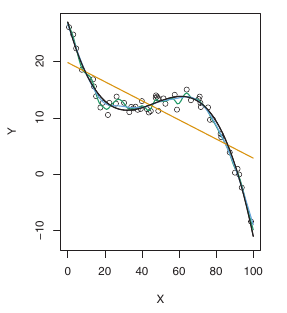
The below figure-A illustrates this phenomenon on a simple example.

In the lefthand panel of Figure A, we have generated observations from
true f given by the black curve. The orange, blue and green curves illus-
trate three possible estimates for f obtained using methods with increasing
levels of flexibility. The orange line is the linear regression fit, which is relatively inflexible. The blue and green curves were produced using smoothing splines. It is clear that as the level of flexibility increases, the curves fit the observed data more closely.
We now move on to the right-hand panel of Figure-A. The grey curve displays the average training MSE as a function of flexibility, or more formally the degrees of freedom, for a number of smoothing splines. The degrees of freedom is a quantity that summarizes the flexibility of a curve.
The test MSE is displayed using the red curve in the right-hand panel of Figure A. As with the training MSE, the test MSE initially declines as the level of flexibility increases. However, at some point the test MSE levels off and then starts to increase again. Consequently, the orange and green curves both have high test MSE. The blue curve minimizes the test MSE, which should not be surprising given that visually it appears to estimate f the best in the lefthand panel of Figure-A
In the right-hand panel of Figure-A, as the flexibility of the statistical learning method increases, we observe a monotone decrease in the training MSE and a U-shape in the test MSE. This is a fundamental property of statistical learning that holds regardless of the particular data set at hand
and regardless of the statistical method being used.
As model flexibility increases, training MSE will decrease, but the test MSE may not.
And when a given method yields a small training MSE but a large test MSE, we are said to be overfitting the data. This happens because our statistical learning procedure is working too hard to find patterns in the training data, and maybe picking up some patterns that are just caused by random chance rather than by true properties of the unknown function f.
However, regardless of whether or not overfitting has occurred, we almost always expect the training MSE to be smaller than the test MSE because most statistical learning methods either directly or indirectly seek to minimize the training MSE.
So now the final point which is The Bias-Variance Trade-Off
The U-shape observed in the test MSE curves in Figure-A above turns out
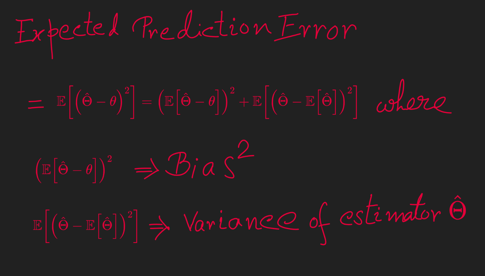
to be the result of two competing properties of statistical learning methods. It is possible to show that the expected test MSE (or sometimes also called Expected Prediction Error ), for a given value x0, can always be decomposed into the sum of three fundamental quantities: the variance of estimated f(x0 ), the squared bias of estimated f(x0 ) and the variance of the error terms.

The left-hand side of the above equation defines the expected test MSE and refers to the average test MSE that we would obtain if we repeatedly estimated f using a large number of training sets, and tested each at x0. The overall expected test MSE can be computed by averaging over all possible values of x0 in the test set
Definition of Variance
The variance of the model is the amount the performance of the model changes or the amount by which the estimated f would change, when it is fit on different training data sets. It captures the impact of the specifics the data has on the model.
Variance informally means how far your data is spread out. Overfitting is you memorizing 10 questions for your exam and on the next day exam, only one question (our of that 10 memorized) has been asked in the question paper. Now you will answer that one question correctly (based on training), but you have no idea what the remaining questions are(Question are HIGHLY VARIED from what you read). In overfitting, the model will memorize the entire train data such that it will give high accuracy on the training-dataset but will fail in test.
For high variance models an alternative is feature reduction (e.g. pruning in Decision Tree, we will cover this in more detail further down in this article), but including more training data is also a viable option. This means when I repeat the entire model building process multiple times, the variance is HOW MUCH THE PREDICTIONS FOR A GIVEN POINT VARY, between different realizations of the model.
Let θ̂ be a point estimator for a parameter θ.
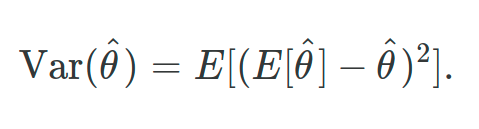
In another form, so you can take a look at the above formula in a slightly different way — the expression of the Variance will be

Where L=100 data sets each with each with N=25
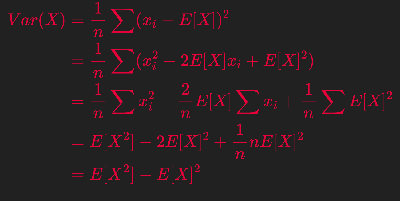
Now take note of an important Mathematical Identity on Variance which is below

And below is the formal proof
Definition of Bias
In the above figure, the true f is substantially non-linear, so no matter how many training observations we are given, it will not be possible to produce an accurate estimate using linear regression. In other words, linear regression results in high bias in this example.
So, the bias is a measure of how close the model can capture the mapping function between inputs and outputs. When a model has a high bias it means that it is very simple and that adding more features should improve it. Bias does not depend on data
So, the error due to bias is taken as the difference between the expected (or average) prediction value from my model and the correct value which I am trying to predict.
Now the basic question is I am only taking one model so how the concept of expected or average prediction values comes here. To understand that, imagine repeating the whole model building process more than once: each time I gather new data and run a new analysis creating a new model. Due to randomness in the underlying data sets, the resulting models will have a range of predictions. So now, the Bias measures how far off these models’ predictions are from the correct value.
So, let θ̂ be a point estimator for a parameter θ. Then θ̂ is an unbiased estimator if E(θ̂ ) = θ, else θ̂ is said to be biased.
The bias of a point estimator θ̂ is given by

If the bias is larger than zero, we also say that the estimator is positively biased, if the bias is smaller than zero, the estimator is negatively biased, and if the bias is exactly zero, the estimator is unbiased.
In another form, for you to take a look at the above Bias formula in a slightly different way — the expression of the Bias will be

Where, just like the alternate expression of Variance, L=100 data sets each with each with N=25
Actual Calculation of Bias
To find the bias of a model (or method), perform many estimates, and add up the errors in each estimate compared to the real value. Dividing by the number of estimates gives the bias of the method. In statistics, there may be many estimates to find a single value. Bias is the difference between the mean of these estimates and the actual value.
High Bias
The two main reasons for high bias are insufficient model capacity and underfitting because the training phase wasn’t complete. For example, if you have a very complex problem to solve (e.g. image recognition) and you use a model of low capacity (e.g. linear regression) this model would have a high bias as a result of the model not being able to grasp the complexity of the problem.
What is an estimator
An estimator is a rule, often expressed as a formula, that tells how to calculate
the value of an estimate based on the measurements contained in a sample.
For example, the sample mean

is one possible point estimator of the population mean μ. Clearly, the expression for ȳ is both a rule and a formula. It tells us to sum the sample observations and divide by the sample size n.
In machine learning, an estimator is an equation for picking the “best,” or most likely accurate, data model based upon observations in realty. Not to be confused with estimation in general, the estimator is the formula that evaluates a given quantity (the estimand) and generates an estimate (source).
Now lets see the process of calculating Estimates


Figure-C below shows two possible sampling distributions for unbiased point estimators for a target parameter θ. We would prefer that our estimator have the type of distribution indicated in Figure C-(b) because the smaller variance guarantees that in repeated sampling a higher fraction of values of θ̂ 2 will be “close” to θ. Thus, in addition to preferring unbiasedness, we want the variance of the distribution of the estimator V (θ̂ ) to be as small as possible. Given two unbiased estimators of a parameter θ, and all other things being equal, we would select the estimator with the smaller variance.

Now for the statistical calculation of this, rather than using the bias and variance of a point estimator to characterize its goodness, we want to employ E[(θ̂ − θ)²], the average of the square of the distance between the estimator and its target parameter.
The mean square error of a point estimator θ̂ is

Below a very popular graph, you will see in many pieces of literature describing the relationship between Bias and Variance.

Some Interpretations from the above Graph
The key Equation of Variance and Bias
MSE(θ̂) = V(θ̂) + [B(θ̂)]²
Which more generally will be below

Bias Variance Tradeoff
There is no escape from the relationship between bias and variance in machine learning which in general is
In short, the bias is the model’s inability to learn enough about the relationship between the model’s features and labels, while the variance captures the model’s inability to generalize on new, unseen examples. A model with high bias oversimplifies the relationship and is said to be underfit. A model with high variance has learned too much about the training data and
is said to be overfit. Of course, the goal of any ML model is to have low bias and low variance but, in practice, it is hard to achieve both. For example, increasing model complexity decreases bias but increases variance, while decreasing model complexity decreases variance but introduces more bias.
However, recent work suggests that when using modern machine learning techniques such as large neural networks with high capacity, this behavior is valid only up to a point. In observed experiments, there is an “interpolation threshold” beyond which very high capacity models are able to achieve zero training error as well as low error on unseen data. Of course, you need much larger datasets in order to avoid overfitting on high capacity models.
The Tradeoff in a Nutshell
Mathematical Derivation of the Bias-Variance Equation
First some Mathematical notation for Expected value calculations for Mean, Variance etc for a sample of data.

If we assume that Y= f( X)+ ϵ and E[ ϵ]=0 and Var( ϵ)= σ², then we we can derive the expression for the expected prediction error of a regression fit

using squared error loss

For notational simplicity let

And recount the below identity that

So now lets Algebraically expand the Expression for Expected Prediction Error
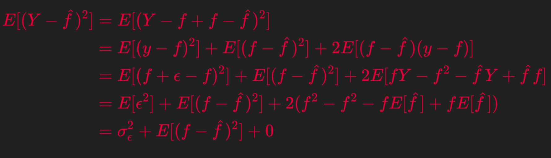
Note in the 4-th line above I have used an
Similarly, expand the second component of the above derivation.
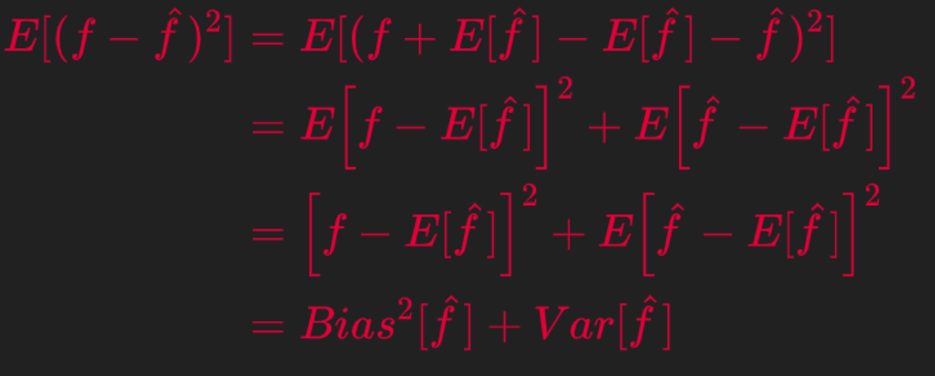
Combining from the above two derivations we get the final relation between Expected Prediction Error on the LHS and the Bias and Variance of the estimator as below.
Now a simple Python Implementation to calculate Bias and Variance
Ways to mitigate this bias-variance tradeoff on small- and medium- scale problems
Ensemble methods to the rescue, which are meta-algorithms which combine several machine learning models as a technique to decrease the bias and/or variance and improve model performance.
Instead of fitting a single final model, you can fit multiple final models. Together, the group of final models may be used as an ensemble. For a given input, each model in the ensemble makes a prediction and the final output prediction is taken as the average of the predictions of the models.
By building several models, with different inductive biases, and aggregating their outputs, we hope to get a model with better performance. Below, we’ll discuss some commonly used Ensemble methods, including bagging, boosting, and stacking.
BAGGING
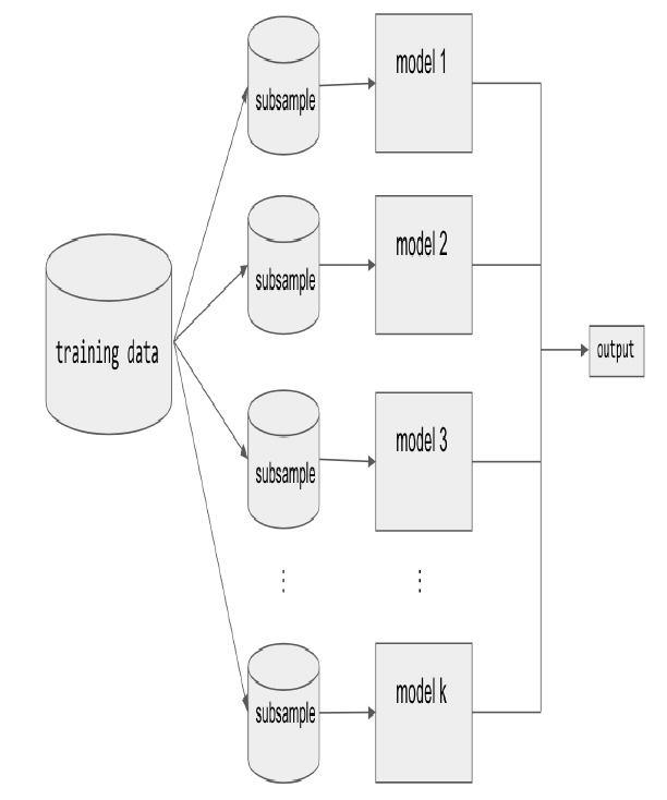
Bagging (short for bootstrap aggregating) is a type of parallel ensembling method and it is used to address high-variance in machine learning models. The bootstrap part of bagging refers to the datasets used for training the ensemble members. Specifically, if there are k sub-model then there are k separate datasets used for training each sub-model of the ensemble. Each dataset is constructed by randomly sampling (with replacement) from the
original training dataset. This means there is a high probability that any of the k datasets will be missing some training examples, but also any dataset will likely have repeated training examples. The aggregation takes place on the output of the multiple ensemble model members, either an average in the case of a regression task or a majority vote in the case of classification. A good example of a bagging Ensemble method is the Random Forest: multiple decision trees are trained on randomly sampled subsets of the entire training data, then the tree predictions are aggregated to produce a prediction, as shown in below Figure.
Most recognized machine learning libraries have implementations of bagging
methods. For example, to implement a Random Forest regression in scikit-learn
Model averaging as seen in bagging is a powerful and reliable method for reducing model variance. Different Ensemble methods combine multiple sub-models in different ways, sometimes using different models, different algorithms, or even different objective functions. With bagging, the model and algorithms are the same. For example, with Random Forest, the submodels are all short Decision Trees.
The next Ensemble technique is BOOSTING
Unlike bagging, boosting ultimately constructs an ensemble model with more capacity than the individual member models. For this reason, boosting provides a more effective means of reducing bias than variance. The idea behind boosting is to iteratively build an Ensemble of models where each successive model focuses on learning the examples the previous model got wrong. In short, boosting iteratively improves upon a sequence of weak learners taking a weighted average to ultimately yield a strong learner.

The next Ensemble technique is STACKING
Stacking is an Ensemble method which combines the outputs of a collection of models to make a prediction. The initial models, which are typically of different model types, are trained to completion on the full training dataset. Then, a secondary meta-model is trained using the initial model outputs as features. This second meta-model learns how to best combine the outcomes of the initial models to decrease the training error and can be any type of machine learning model.
An example of reducing Variance of a Decision Tree
A decision tree has high variance because, if you imagine a very large tree, it can basically adjust its predictions to every single input.
Consider you wanted to predict the outcome of a Cricket game. A decision tree could make decisions like:
If the tree is very deep, it will get very specific and you may only have one such game in your training data. It probably would not be reasonable to base your predictions on just one example.
Now, if you make a small change e.g. set the number of attending fans to 25999, a decision tree might give you a completely different answer (because the game now doesn’t meet the 4th condition).
Linear regression, for example, would not be so sensitive to a small change because it is limited (or “biased” ) to linear relationships and cannot represent sudden changes from 25999 to 26000 fans.
That’s why it is important to not make decision trees arbitrary large/deep. This limits its variance.
This is why we usually use pruning for avoiding the trees to get overfitted to the training data. Pruning reduces the size of decision trees by removing parts of the tree that do not provide power to classify instances. One way can be ignoring some features and using others. Pruning is computationally inexpensive, reduces complexity significantly, and variance to some extent, but also increases bias.
Let’s implement the above with a quick numerical example with Scikit-learn to see how Variance Reduction is achieved by Pruning a Decision Tree but with the cost of Increased Bias.