The T-tests are performed to compute the confidence limits for one sample or two independent samples by comparing their means and mean differences. The SAS procedure named PROC TTEST is used to carry out t tests on a single variable and pair of variables.
Syntax
The basic syntax for applying PROC TTEST in SAS is −
Following is the description of the parameters used −
Dataset is the name of the dataset.
Variable_1 and Variable_2 are the variable names of the dataset used in t test.
Example
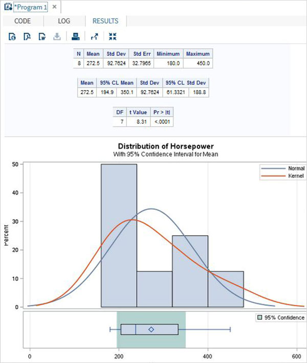
Below we see one sample t test in which find the t test estimation for the variable horsepower with 95 percent confidence limits.
When the above code is executed, we get the following result −
Paired T-test
The paired T Test is carried out to test if two dependent variables are statistically different from each other or not.
Example
As length and weight of a car will be dependent on each other we apply the paired T test as shown below.
When the above code is executed, we get the following result −

Two sample t-test
This t-test is designed to compare means of same variable between two groups.
Example
In our case we compare the mean of the variable horsepower between the two different makes of the cars(«Audi» and «BMW»).
When the above code is executed, we get the following result −
Тест статистической значимости в SAS
Дата публикации Aug 20, 2019

Многие материалы доступны для проверки статистической значимости. Этот блог дает вам краткое представление о том, почему, что, когда и как использовать статистический тест? Кроме того, этот пост является попыткой быстрого пересмотра использования этих статистических тестов. Значение p и гипотеза не обсуждались в этом блоге, и вы можете проверитьВот,
Зачем нам нужно много статистических тестов?

Например, мы хотим измерить вес мяча. У нас есть четыре устройства для измерения, такие как физический баланс, термометр, линейка и мерная колба. Какой из них мы выбираем? Очевидно, мы выбираем физическое равновесие. Не так ли? Предположим, мы хотим измерить температуру мяча? Затем выбираем термометр. Для объема, затем выбираем мерную колбу.
Теперь вы можете видеть, что в качестве переменной, которую мы хотим измерить, изменяется и устройство. Точно так же, почему у нас так много статистических тестов? У нас есть разные типы переменных и анализа. По мере изменения типа анализа меняются и статистические тесты.
Давайте возьмем другой пример. Предположим, Учитель хочет сравнить рост мальчиков и девочек в классе.

Так Учитель порождает Нулевую и Альтернативную Гипотезу. Вот,
Нулевая гипотеза (H0)→ Рост мальчиков и девочек одинаков, и любое различие между высотами случайно.
Альтернативная гипотеза (H1)→ Рост мальчиков выше, чем рост девочек, поэтому наблюдаемые различия между ростом реальны.
Как проверить эту гипотезу? Для этого играет роль критерий статистической значимости.

Что такое тест статистической значимости?
Это тест, который помогает исследователям или аналитикам подтвердить гипотезу. Другими словами, эти тесты помогают, является ли гипотеза верной или нет?
Есть много статистических тестов. Но мы увидим два типа в этом блоге.
Тест статистической значимости делится на два типа.

Следующий вопрос, когда использовать?

Выбор статистического теста
Как параметрические, так и непараметрические тесты имеют разные виды тестов (различные типы параметрических тестов были рассмотрены ниже), но как аналитик или исследователь выбирает правильный тест на основе дизайна исследования, типа переменной и распределения?
Приведенная ниже таблица содержит краткое изложение вопросов, на которые необходимо ответить перед выбором правильного теста. Справка: Университет Миннесоты. Ты можешь проверитьВот,

Что такое параметрический тест?
Используется, если информация о населении полностью известна посредством ее параметров, тогда статистический тест называется параметрическим тестом.
Типы параметрического теста
1) t-тест
T-тест для одного образца
T-критерий сравнивает разницу между двумя средними значениями в разных группах, чтобы определить, является ли разница статистически значимой

Давайте возьмем пример набора данных hbs2. Набор данных содержит 200 наблюдений из выборки старшеклассников. Он имеет пол, социально-экономический статус, этническое происхождение, такие предметы, как чтение, письмо, математика, общественные науки.


Здесь хотелось бы проверить, отличается ли средняя оценка письма от 50.

Здесь значение р составляет менее 0,05. Следовательно, среднее значение переменной записи для этой выборки студентов составляет 52,77, что статистически значительно отличается от значения теста 50. Мы пришли бы к выводу, что эта группа студентов имеет значительно более высокое среднее значение по тесту письма, чем 50.
t-тест для двух образцов
Он используется, когда две независимые случайные выборки происходят из нормальных популяций, имеющих неизвестную или одинаковую дисперсию. Он разделен на два типа
Независимый выборочный t-критерий используется, когда вы хотите сравнить средние значения нормально распределенной переменной, зависящей от интервала, для двух независимых групп. Другими словами, этот t-критерий предназначен для сравнения средних значений одной и той же переменной между двумя группами.


2. Парный t-критерий с двумя образцами
Он используется, когда у вас есть два связанных наблюдения (то есть два наблюдения на субъекта), и вы хотите увидеть, отличаются ли средние значения этих двух нормально распределенных интервальных переменных друг от друга.

Проверка письма и чтения

Значение р> 0,05. Приведенный выше результат показывает, что среднее значение чтения статистически не отличается от среднего значения записи.
2) Z-тест
Z-критерий представляет собой статистический критерий, в котором применяется нормальное распределение и в основном используется для решения проблем, связанных с большими выборками, когда частота больше или равна 30. Он используется, когда известно стандартное отклонение совокупности. Если размер выборки меньше 30, тогда применяется t-критерий.
В SAS proc t-test позаботится о размере выборки и даст соответствующие результаты. В SAS нет отдельного кода для z-теста.
3) Анализ отклонений (ANOVA)
Это набор статистических моделей, используемых для анализа различий между групповыми средними или отклонениями.
Односторонний ANOVA
Односторонний дисперсионный анализ (ANOVA) используется, когда у вас есть категориальная независимая переменная (с двумя или более категориями) и нормально распределенная переменная, зависящая от интервала, и вы хотите проверить различия в средствах зависимой переменной с разбивкой по: уровни независимой переменной.
В SAS это делается с помощьюПРОЦ АНОВА


Двухсторонний ANOVA

Здесь запишите в качестве зависимой переменной и женский и социально-экономический статус (ы) в качестве независимых переменных. Мы хотели бы проверить, написание отличается между женщиной и сес.

Эти результаты показывают, что общая модель является статистически значимой (F = 8,39, р = 0,0001). Переменныеженщинаа такжесесявляются статистически значимыми (F = 14,55, р = 0,0002 и F = 5,31, р = 0,0057 соответственно).
4) корреляция Пирсона (r)
Корреляция полезна, когда вы хотите увидеть линейную связь между двумя (или более) нормально распределенными переменными интервала.
Мы можем установить корреляцию между двумя непрерывными переменными чтения и записи в нашем наборе данных


Мы можем видеть, что корреляция междучитатьа такжезаписывать0,59678. Вычисляя корреляцию, а затем умножая на 100, мы можем узнать, какой процент изменчивости является общим. Пусть округление 0,59678 до 0,6, что при квадрате равно 0,36, умноженное на 100, составит 36%. следовательночитать акцииоколо 36% его изменчивости сзаписывать,
Я объясню Непараметрический тест в моей следующей статье.
Продолжайте учиться и следите за обновлениями!
SAS — T Тесты
T-тесты выполняются для вычисления доверительных интервалов для одного или двух независимых образцов путем сравнения их средних и средних различий. Процедура SAS с именем PROC TTEST используется для проведения t-тестов для одной переменной и пары переменных.
Синтаксис
Основной синтаксис применения PROC TTEST в SAS —
Ниже приведено описание используемых параметров:
Набор данных — это имя набора данных.
Переменная_1 и Переменная_2 — это имена переменных набора данных, используемого в t-тесте.
Набор данных — это имя набора данных.
Переменная_1 и Переменная_2 — это имена переменных набора данных, используемого в t-тесте.
пример
Ниже мы видим один пример t-теста, в котором находят оценку t-теста для переменной мощности с 95-процентным доверительным интервалом.
Когда приведенный выше код выполняется, мы получаем следующий результат —

Парный Т-тест
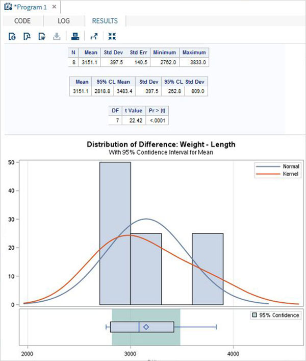
Парный T-тест проводится для проверки того, являются ли две зависимые переменные статистически отличными друг от друга или нет.
пример
Поскольку длина и вес автомобиля будут зависеть друг от друга, мы применяем парный Т-тест, как показано ниже.
Когда приведенный выше код выполняется, мы получаем следующий результат —
Два образца t-теста
Этот t-тест предназначен для сравнения средних значений одной и той же переменной между двумя группами.
пример
В нашем случае мы сравниваем среднее значение переменной мощности для двух разных марок автомобилей («Ауди» и «БМВ»).
Когда приведенный выше код выполняется, мы получаем следующий результат —
Proc TTest | SAS Annotated Output
The ttest procedure performs t-tests for one sample, two samples and paired observations. The single-sample t-test compares the mean of the sample to a given number (which you supply). The dependent-sample t-test compares the difference in the means from the two variables to a given number (usually 0), while taking into account the fact that the scores are not independent. The independent samples t-test compares the difference in the means from the two groups to a given value (usually 0). In other words, it tests whether the difference in the means is 0. In our examples, we will use the hsb2 data set.
Single sample t-test
For this example, we will compare the mean of the variable write with a pre-selected value of 50. In practice, the value against which the mean is compared should be based on theoretical considerations and/or previous research.
Summary statistics
a. Variable – This is the list of variables. Each variable that was listed on the var statement will have its own line in this part of the output.
b. N – This is the number of valid (i.e., non-missing) observations used in calculating the t-test.
c. Lower CL Mean and Upper CL Mean – These are the lower and upper bounds of the confidence interval for the mean. A confidence interval for the mean specifies a range of values within which the unknown population parameter, in this case the mean, may lie. It is given by
d. Mean – This is the mean of the variable.
e. Lower CL Std Dev and Upper CL Std Dev – Those are the lower and upper bound of the confidence interval for the standard deviation. A confidence interval for the standard deviation specifies a range of values within which the unknown parameter, in this case, the standard deviation, may lie. The computation of the confidence interval is based on a chi-square distribution and is given by the following formula
where S 2 is the estimated variance of the variable and alpha is the confidence level. If we drew 200 random samples, then about 190 (200*.95) of times, the confidence interval would capture the parameter standard deviation of the population.
f. Std Dev – This is the standard deviation of the variable.
g. Std Err – This is the estimated standard deviation of the sample mean. If we drew repeated samples of size 200, we would expect the standard deviation of the sample means to be close to the standard error. The standard deviation of the distribution of sample mean is estimated as the standard deviation of the sample divided by the square root of sample size. This provides a measure of the variability of the sample mean. The Central Limit Theorem tells us that the sample means are approximately normally distributed when the sample size is 30 or greater.
Test statistics
a. Variable – This is the list of variables. Each variable that was listed on the var statement will have its own line in this part of the output. If a var statement is not specified, proc ttest will conduct a t-test on all numerical variables in the dataset.
h. DF – The degrees of freedom for the single sample t-test is simply the number of valid observations minus 1. We loose one degree of freedom because we have estimated the mean from the sample. We have used some of the information from the data to estimate the mean; therefore, it is not available to use for the test and the degrees of freedom accounts for this.
i. t Value – This is the Student t-statistic. It is the ratio of the difference between the sample mean and the given number to the standard error of the mean. Since that the standard error of the mean measure the variability of the sample mean, the smaller the standard error of the mean, the more likely that our sample mean is close to the true population mean. This is illustrated by the following three figures.
All three cases the difference between the population means are the same. But with large variability of sample means, two populations overlap a great deal. Therefore, the difference may well come by chance. On the other hand, with small variability, the difference is more clear. The smaller the standard error of the mean, the larger the magnitude of the t-value. Therefore, the smaller the p-value. The t-value takes into account of this fact.
Dependent group t-test
Summary statistics
a. Difference – This is the list of variables.
b. N – This is the number of valid (i.e., non-missing) observations used in calculating the t-test.
c. Lower CL Mean and Upper CL Mean – These are the lower and upper bounds of the confidence interval for the mean. A confidence interval for the mean specifies a range of values within which the unknown population parameter, in this case the mean, may lie. It is given by
d. Mean – This is the mean of the variable.
e. Lower CL Std Dev and Upper CL Std Dev – Those are the lower and upper bound of the confidence interval for the standard deviation. A confidence interval for the standard deviation specifies a range of values within which the unknown parameter, in this case, the standard deviation, may lie. The computation of the confidence interval is based on a chi-square distribution and is given by the following formula
where S 2 is the estimated variance of the variable and alpha is the confidence level. If we drew 200 random samples, then about 190 (200*.95) of times, the confidence interval would capture the parameter standard deviation of the population.
f. Std Dev – This is the standard deviation of the variable.
g. Std Err – This is the estimated standard deviation of the sample mean. If we drew repeated samples of size 200, we would expect the standard deviation of the sample means to be close to the standard error. The standard deviation of the distribution of sample mean is estimated as the standard deviation of the sample divided by the square root of sample size. This provides a measure of the variability of the sample mean. The Central Limit Theorem tells us that the sample means are approximately normally distributed when the sample size is 30 or greater.
Test statistics
h. Difference – The t-test for dependent groups is to form a single random sample of the paired difference. Therefore, essentially it is a simple random sample test. The interpretation for t-value and p-value is the same as for the case of simple random sample.
i. DF – The degrees of freedom for the paired observations is simply the number of observations minus 1. This is because the test is conducted on the one sample of the paired differences.
j. t Value – This is the t-statistic. It is the ratio of the mean of the difference in means to the standard error of the difference (.545/.6284).
k. Pr > |t| – The p-value is the two-tailed probability computed using t distribution. It is the probability of observing a greater absolute value of t under the null hypothesis. For a one-tailed test, halve this probability. If p-value is less than our pre-specified alpha level, usually 0.05, we will conclude that the difference is significantly from zero. For example, the p-value for the difference between write and read is greater than 0.05, so we conclude that the difference in means is not statistically significantly different from 0.
Independent group t-test
This t-test is designed to compare means of same variable between two groups. In our example, we compare the mean writing score between the group of female students and the group of male students. Ideally, these subjects are randomly selected from a larger population of subjects. Depending on if we assume that the variances for both populations are the same or not, the standard error of the mean of the difference between the groups and the degree of freedom are computed differently. That yields two possible different t-statistic and two different p-values. When using the t-test for comparing independent groups, we need to test the hypothesis on equal variance and this is a part of the output that proc ttest produces. The interpretation for p-value is the same as in other type of t-tests.
Summary statistics
a. Variable – This column lists the dependent variable(s). In our example, the dependent variable is write.
b. female – This column gives values of the class variable, in our case female. This variable is necessary for doing the independent group t-test and is specified by class statement.
c. N – This is the number of valid (i.e., non-missing) observations in each group defined by the variable listed on the class statement (often called the independent variable).
d. Lower CL Mean and Upper CL Mean – These are the lower and upper confidence limits of the mean. By default, they are 95% confidence limits.
e. Mean – This is the mean of the dependent variable for each level of the independent variable. On the last line the difference between the means is given.
f. Lower CL Std Dev and Upper LC Std Dev – These are the lower and upper 95% confidence limits for the standard deviation for the dependent variable for each level of the independent variable.
g. Std Dev – This is the standard deviation of the dependent variable for each of the levels of the independent variable. On the last line the standard deviation for the difference is given.
h. Std Err – This is the standard error of the mean.
Test statistics
a. Variable – This column lists the dependent variable(s). In our example, the dependent variable is write.
i. Method – This column specifies the method for computing the standard error of the difference of the means. The method of computing this value is based on the assumption regarding the variances of the two groups. If we assume that the two populations have the same variance, then the first method, called pooled variance estimator, is used. Otherwise, when the variances are not assumed to be equal, the Satterthwaite’s method is used.
j. Variances – The pooled estimator of variance is a weighted average of the two sample variances, with more weight given to the larger sample and is defined to be
s 2 = ((n1-1)s1+(n2-1)s2)/(n1+n2-2),
Satterthwaite is an alternative to the pooled-variance t test and is used when the assumption that the two populations have equal variances seems unreasonable. It provides a t statistic that asymptotically (that is, as the sample sizes become large) approaches a t distribution, allowing for an approximate t test to be calculated when the population variances are not equal.
k. DF – The degrees of freedom for the paired observations is simply the number of observations minus 2. We use one degree of freedom for estimating the mean of each group, and because there are two groups, we use two degrees of freedom.
l. t Value – This t-test is designed to compare means between two groups of the same variable such as in our example, we compare the mean writing score between the group of female students and the group of male students. Depending on if we assume that the variances for both populations are the same or not, the standard error of the mean of the difference between the groups and the degrees of freedom are computed differently. That yields two possible different t-statistic and two different p-values. When using the t-test for comparing independent groups, you need to look at the variances for the two groups. As long as the two variances are close (one is not more than two or three times the other), go with the equal variances test. The interpretation for the p-value is the same as in other types of t-tests.
m. Pr > |t| – The p-value is the two-tailed probability computed using the t distribution. It is the probability of observing a t-value of equal or greater absolute value under the null hypothesis. For a one-tailed test, halve this probability. If the p-value is less than our pre-specified alpha level, usually 0.05, we will conclude that the difference is significantly different from zero. For example, the p-value for the difference between females and males is less than 0.05, so we conclude that the difference in means is statistically significantly different from 0.
n. Num DF and Den DF – The F distribution is the ratio of two estimates of variances. Therefore it has two parameters, the degrees of freedom of the numerator and the degrees of freedom of the denominator. In SAS convention, the numerator corresponds to the sample with larger variance and the denominator corresponds to the sample with smaller variance. In our example, the male students group ( female=0) has variance of 10.305^2 (the standard deviation squared) and for the female students the variance is 8.1337^2. Therefore, the degrees of freedom for the numerator is 91-1=90 and the degrees of freedom for the denominator 109-1=108.
o. F Value – SAS labels the F statistic not F, but F’, for a specific reason. The test statistic of the two-sample F test is a ratio of sample variances, F = s1 2 /s2 2 where it is completely arbitrary which sample is labeled sample 1 and which is labeled sample 2. SAS’s convention is to put the larger sample variance in the numerator and the smaller one in the denominator. This is called the folded F-statistic,
which will always be greater than 1. Consequently, the F test rejects the null hypothesis only for large values of F’. In this case, we get 10.305^2 / 8.1337^2 = 1.605165, which SAS rounds to 1.61.
p. Pr > F – This is the two-tailed significance probability. In our example, the probability is less than 0.05. So there is evidence that the variances for the two groups, female students and male students, are different. Therefore, we may want to use the second method (Satterthwaite variance estimator) for our t-test.
Primary Sidebar
Click here to report an error on this page or leave a comment